Grafana – kdb+ adaptor

AquaQ Analytics are often involved in projects using different visualisation tools connected to kdb+.  We have recently spent some time reviewing and then implementing a simple Grafana-kdb+ adaptor. This open-source script has been developed using the inbuilt Grafana SimpleJSON datasource and comes with the capability of table and time series visualisation and manipulation. Instructions for installation and usage can be found in this article with additional information on the development process and steps going forward. If you would like to discuss any kdb+ visualisation project, you can contact us: info@aquaq.co.uk.

Grafana for kdb+

Grafana is an open-source analytics platform, used to display time series data from a web application. Currently it supports a variety of datasources including Graphite, InfluxDB & Prometheus with users including the likes of PayPal, eBay, Intel and Booking.com.  However, there is no in-built support for direct analysis of data from kdb+. Thus, using the SimpleJSON datasource, we have engineered an adaptor to allow visualisation of kdb+ data.

The Grafana-kdb+ adaptor

The SimpleJSON datasource operates by sending query requests directly from Grafana as an HTTP POST request. Consequently, the connection is held until a result is returned from the handle.  This forms the basis for our adaptor. When a request is made on the Grafana web application, the request is sent to the port at which the datasource is set.  The request is delivered as a string in JSON format of the request and a dictionary of Grafana-based information.

This request string can be handled in kdb+ by using the inbuilt function .j.k, creating a dictionary of the enclosed information. The request string has a prefix of one of six urls. Four mandatory urls needed for the adaptor to work are /, /search, /query and /annotation while /tag-keys and /tag-values are optional extras. For example given the /query request in 

"search {\"target\":\"\"}"
"query {\"timezone\":\"browser\",\"panelId\":1,\"dashboardId\":null,..

the url of the request is stated before the JSON dictionary. Recognising each url in a request allows us to manipulate what is displayed on the Grafana browser. For instance, /search controls what options are displayed in the drop down menu while /query enters the selected option into the main body of our adaptor. Within this main body, the query is executed on the kdb+ instance, the data selected, formatted back to JSON and displayed within the dashboard. From here there is a full range of Grafana-based data manipulation available directly through the browser.

From the /query request example above we obtain the q dictionary in JSON format:

{
  "timezone":"browser",
  "panelId":1,
  "dashboardId":null,
  "range":{
    "from":"2018-09-24T08:58:26.149Z",
    "to":"2018-09-24T09:03:26.149Z",
    "raw":{"from":"now-5m","to":"now"}
  },
  "rangeRaw":{"from":"now-5m","to":"now"},
  "interval":"2s",
  "intervalMs":2000,
  "targets":[{"target":"o.trade.price.NYSE","refId":"A","type":"timeserie"}],
  "maxDataPoints":100,
  "scopedVars":{
    "__interval":{"text":"2s","value":"2s"},
    "__interval_ms":{"text":"2000","value":"2000"}
  },
  "cacheTimeout":null,
  "adhocFilters":[]
}

Each section of the request can be accessed through keys in this dictionary. In this case, all of the relevant query information can be found in the targets entry with the time manipulation found in range. Upon closer inspection of range and targets we can see the sub-dictionaries are contained within braces in our query.

The key elements to extract from these sub-dictionaries are the request type, table or time series, and the actual query to run. From this request a kdb+ query is executed and the result formatted to fit the SimpleJSON response template for either table or time series.

The dictionary of Grafana-based information from SimpleJSON always has the format

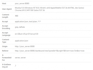
where the information is interchangeable for each user. This dictionary is used only for checks that the HTTP POST request is from Grafana so we will not discuss it here.

The adaptor uses HTTP request handlers .z.pp and .z.ph. To ensure the current .z.* are not overwritten by use of the adaptor, these functions have been defined within a wrapper and our custom .z.* is called only in the circumstance that the call is from Grafana. Our adaptor also includes customisable configuration settings. Such configurations include user customisation of the standard time and sym column names and can be found at the head of the adaptor’s code.

Setting up

To get started with using this adaptor you will have to first set up Grafana. This is well explained on the Grafana website where you have the option to either download the software locally or let Grafana host it for you. It is also necessary to install the SimpleJSON plugin from the Grafana plugin directory. From there you must log onto Grafana and set up a SimpleJSON datasource with the url including the kdb+ port your data is hosted on. On the kdb+ side you must download our adaptor grafana.q from AquaQ’s TorQ git repository and load the file into the q session with the data. Note that grafana.q works both within the TorQ system and as standalone code. If using Grafana to visualise data straight from a RDB or HDB in TorQ then it is also necessary for access credentials to be inputted on the Grafana datsource set-up page.

Using the adaptor

Note: All data in here is from fake data.

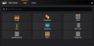
Our adaptor aims to encapsulate all the functionality provided by a native datasource. Panels can be added to a dashboard using the ‘New Panel’ tab. The options for these panels can be seen below, the most common being graph and table.

Once a panel has been selected the user can then supply their given query in the metrics section. The options for such queries are automatically populated as can be seen here:

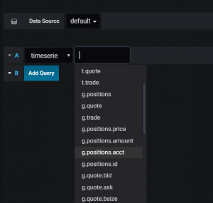
As the JSON message does not return the type of panel selected, the drop down is populated with all possible query options for the tables within the data. To distinguish between the panels, options for each query starts with either ‘t’, ‘g’ or ‘o’ representing table, graph or other. The option chosen will then define the body of the query. The logic of this can be seen here:

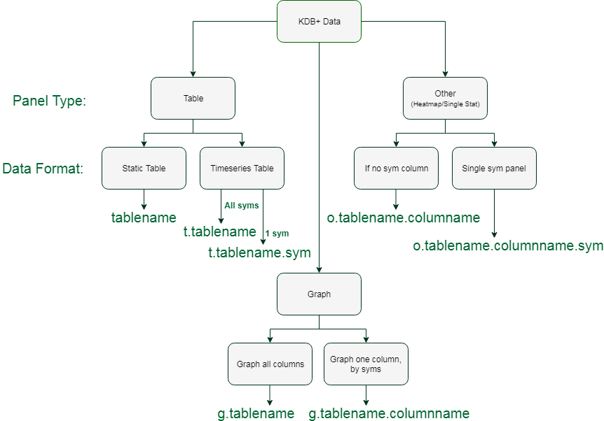
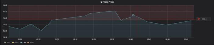
This format allows the processing of static tables, as well as time series tables, graphs, heatmaps and statistics. The tabular input, t.tablename.sym, supports selection of data for a given sym from a table. Graphs can be created displaying a given column for each sym using the t.tablename.columnname convention. Although this query returns each sym, they can then be isolated using the legend of the graph to display either one or all, as can be seen below:

With these panels in place the usual Grafana functionality can be utilised. For example:

• Tabular data can be manipulated to alter precision, types or include units.
• Unwanted columns can be hidden.
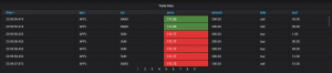
• Tables can be given a threshold to colour co-ordinate prices:

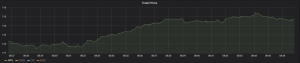
Graphs can be used to set alert systems (e.g. if the price of a sym drops below a given threshold):

In addition to graph and table panel functionality, there is an option for ‘other’. This option allows for use of the heatmap and single stat panels which only accept one data string:

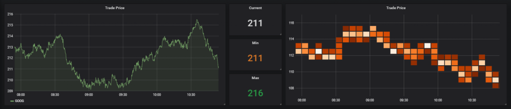
Note, this option also functions within the graph panel but will return one line only.

Capabilities and Limitations

The combination of Grafana and our adaptor facilitates the visualisation of a wide range of data structures. However, in addition to being built for both in-memory and on-disk data there are several other limitations to the permitted inputs:

• Data Refresh: The adaptor handles real-time databases with negligible lag. However, Grafana has a default minimum refresh option of 5 seconds causing a latent stream from the datasources.
• Time Accuracy: The SimpleJSON plugin expects all time series data to be returned with the time format of milliseconds since 1970.01.01. This limits all data coming in from the feed to only millisecond precision which may not be suitable for some time series data.
• Data Size: As a free, open-source visualisation software Grafana offers a generous amount of data hosting and active datasources with the base level being 2 servers and 18,000 data points per minute. In addition it offers up to 50,000 servers, 45,000,000 data points per minute and two years data retention for the right price.

Going forward

SimpleJSON has yielded far more results than we initially thought possible and offers us easy access to data already available on the kdb+ server. However, in future adaptor development, it may be needed to branch out and explore other datasources or build a kdb+ specific datasource. SimpleJSON is limited in that it only allows a singular drop down option, with the panel type not being specified within the request. Other viable options would be using the Graphite datasource where our adaptor would need little alteration due to its ability to use JSON formatting and the ability to utilise multiple drop downs. This form of adaptor could simplify the code and enable a friendlier user interface to be created. In addition, due to the SQL-like qSQL statements within q then InfluxDB and PostgreSQL are other datasources to consider.