AquaQ's BigQuery API: Accessing Google's BigQuery Data in kdb+

Introduction

Google’s BigQuery is a fully scalable, serverless, cloud data warehouse of ever-increasing popularity. It boasts impressive ease of use as well as low-cost, quick configuration and “super-fast”[1] SQL querying across data. Making use of worker processes (like kdb+ secondary processes) and Google’s processing infrastructure, BigQuery’s querying speeds tower above many other SQL data warehouses. For a SQL-based storage and querying solution, BigQuery performs incredibly well.

As a result of these benefits, Google’s platform is gaining more and more traction in financial industries. In confirmation of this, Refinitiv has uploaded data containing over the counter and exchange-traded instruments from all asset classes in more than 500 venues dating back to 1996[2]. This means that, Refinitiv’s customers have access to the full extent of their historical tick data drawn from real-time content. AquaQ Analytics have been working with Refinitiv in order to develop the interface as described in this blog.

kdb+, like BigQuery, has a lot of positive attributes associated with it, but how do they compare to each other? BigQuery draws a lot of acclaim from its cheap storage and commendable querying speeds. Whereas, kdb+ offers significant improvement on BigQuery’s querying speeds but users are left with the expensive cost of on-disk storage. Therefore, users face the apparent options of sacrificing cheap storage for fast querying with kdb+, or sacrificing faster querying for cheaper storage with BigQuery. AquaQ Analytics has been developing a more dynamic model in which users can draw benefits from both databases.

Architecture

AquaQ’s BigQuery API is one of data-access that allows the querying of data within BigQuery, as well as extraction and conversion of the data into kdb+. The API can be run in either a “stand-alone” set-up, or can be used in conjunction with kdb+ processes such as real-time and historical databases within TorQ (AquaQ’s open sourced kdb+ extended tick framework). Just as the target application, the BigQuery API has been designed to have as little setup as possible for the user and requires only a few configuration files to be set-up in order to query data.

The stand-alone configuration is designed so that users have an easy method for querying their data from kdb+. Users can query with either raw SQL inputs or with kdb+ input dictionaries that generate the SQL queries for the user. This is the SQL forming equivalent to the data access API as described in a previous blogpost by AquaQ: Data Access API.

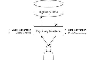
The BigQuery interface stand-alone set-up

As the diagram above shows, the standalone set-up is a simple one and allows a user to directly interact with the kdb+ living BigQuery interface process in order to receive their BigQuery stored data. The stand-alone set-up is not restricted to use within TorQ and can be easily slotted into a user’s predefined architecture. The code requires little configuration and has the option for redefining logic (typically around logging) so that the process fits seamlessly into an existing code base.

The process as described so far is supplemented by many different forms of extra functionality. Four major components of this added versatility (listed in the diagram above) are slightly expanded upon below.

Query checks – the interface provides detailed checking of all inputs so that errors are returned both quickly and insightfully.
Query generation – the process is user-friendly for users both experienced and unexperienced in SQL querying. Queries can be generated from a kdb+ input dictionary or from straight SQL input.
Data conversion – naturally, the return of the data from BigQuery sees type conversion into kdb+ data types.
Post-processing – before data is returned to the user, kdb+ post-processing options are granted. Users have both SQL and kdb+ at their disposal for querying in this sense.

For users of TorQ, the process extends the well-defined tick set-up to allow for everything defined in the stand-alone structure. At the same time, it allows users to query across other kdb+ processes and join the results together. This leads to a dynamic data storage solution that can address the problem set out previously. This resultant storage architecture resembles the diagram below.

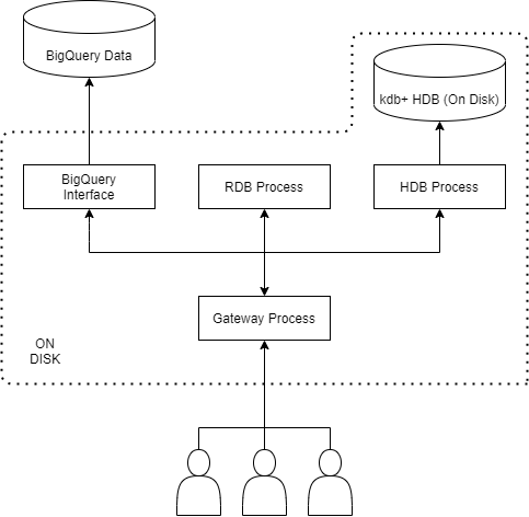
This image has an empty alt attribute; its file name is bqdiagram.png — The structure of BigQuery Interface Process extending the TorQ framework

This solution allows users to have their newest, and likely most frequently accessed, data to be stored in a kdb+ Historical Database (HDB) or Realtime Database (RDB) for quick querying. All the while, having their older, less frequently accessed, data stored in Google’s BigQuery for cheaper storage with slightly slower querying speeds. Users are not impeded by an abandonment of one quality for another; but rather, can yield both quick querying speeds and small storage costs in order to advance their data storage architecture.

Querying Against Refinitiv’s BigQuery Data Store

Unsurprisingly, the BigQuery API enables the straight passing of SQL statements into BigQuery in order to retrieve data into kdb+. The API performs the conversion of BigQuery’s SQL datatypes into their most similar kdb+ datatypes. However, the API is more powerful than simply swapping raw SQL querys for corresponding data. The API can generate SQL query strings using a simple input dictionary of parameters in kdb+. Meaning that a user does not require any knowledge of SQL (and admittedly, fairly little knowledge of kdb+ outside of creating simple dictionaries) in order to query their data.

The input dictionary centres around a simplistic set of keys, each of which relates to a different property of the final query. Such a dictionary may look as follows:

tablename   | `quote
starttime   | 2020.01.01D08:00:00.000000000
endtime     | 2020.01.02D12:00:00.000000000
aggregations| `max`min`avg!`bid`bid`bid
grouping    | `sym
ordering    | `asc`sym

Which corresponds to the following SQL statement:

SELECT
  sym,
  MAX(bid) AS maxBid,
  MIN(bid) AS minBid,
  AVG(bid) AS avgBid
FROM
  `projectName.datasetName.quote`
WHERE
  date BETWEEN '2020-01-01'
  AND '2020-01-02'
  AND time BETWEEN '2020-01-01 08:00:00.000000 UTC'
  AND '2020-01-02 12:00:00.000000 UTC'
GROUP BY
  sym
ORDER BY
  sym

Here the code knows to target the partitioning date column in the where clause before the time column to improve querying speeds and reduce user costs. The ordering of the where clause applies to any clustering columns also, in order to make sure the user is getting the fastest and cheapest query possible.

These simple seeming SQL queries can grow in complexity as different parameters are included within the input dictionary. For example, adding a timebar parameter enables the user to perform aggregations over chosen time-buckets of data. Furthermore, generation of first and last aggregations is possible with the input dictionary (a relatively difficult task in SQL when compared to such queries in kdb+). The API automatically creates the relevant sub-tables in order to perform this SQL complex query. Nevertheless, users have the option of generating the queries themselves or having the process generate the query for them.

As mentioned previously, the markets data provider Refinitiv, has a large amount of data living in BigQuery. This means that customer’s of Refinitiv can query against this large data platform in order to have access to all the data they need, without having to worry about the cost of storage.

One such table in Refinitiv’s dataset revolves around normalised London Stock Exchange Data (aptly named LSE_NORMALISED), is over 27 Terabytes in size and has been used as the subject of some testing for the BigQuery interface process. Suppose that the following query was desired to be run:

SELECT 
    RIC,
    AVG(Price) AS avgPrice,
    SUM(Volume) AS sumVolume,
    COUNT(RIC) AS countRIC
FROM 
    `dbd-sdlc-prod.LSE_NORMALISED.LSE_NORMALISED`
WHERE 
    DATE(Date_Time) = '2021-02-01'
    AND RIC LIKE '{e673f69332cd905c29729b47ae3366d39dce868d0ab3fb1859a79a424737f2bd}.L'
    AND Type = 'Trade'
GROUP BY 
    RIC
ORDER BY 
    countRIC DESC

In order to calculate the average of Price, the sum of Volume, the count of RIC by RIC for the date 2021.02.01, only selecting RICs that end in “.L” and Types equating to “Trade”. This query can be performed through the API (below used in stand-alone format) in a couple of different ways. The query can be written out explicitly as a string and passed into the getdata function as follows:

q)getdata `sqlquery`postprocessing!(queryString;{xkey[`RIC`Type;x]})
RIC    | AvgPrice sumVolume countRIC
-------| ---------------------------
BP.L   | 268.3059 65505660  33136
POLYP.L| 1684.375 3773921   23609
AZN.L  | 7362.532 3391364   23068
RIO.L  | 5600.727 2273576   18169
..

Here queryString represents the query above as a kdb+ string. The postprocessing argument needs to be added to the input dictionary otherwise the table will be returned unkeyed. This is due to the fact that, the concept of a keyed table does not align over the two languages and the table is otherwise returned as a simple table.

This table can also be produced via the input dictionary method by taking a dictionary as seen below.

q)queryDictionary
tablename    | `LSE_NORMALISED
starttime    | 2021.02.01
endtime      | 2021.02.01
timecolumn   | `Date_Time
aggregations | `avg`sum`count!`Price`Volume`RIC
freeformwhere| "RIC like \"*.L\",Type=`Trade"
grouping     | `RIC
ordering     | `desc`countRIC

Here it is seen that the freeformwhere parameter grants users the option to type out a where clause in qSQL; users have the option to use either this format or a dictionary format in a parameter called filters. The input dictionary can be used in the functions .bq.getsqlquery and getdata in order to see the query generated by the process and run the query respectively.

q).bq.getsqlquery queryDictionary
"SELECT RIC, AVG(Price) AS avgPrice, SUM(Volume) AS sumVolume, COUNT(RIC) AS countRIC FROM `dbd-sdlc-prod.LSE_NORMALISED.LSE_NORMALISED` WHERE DATE(Date_Time) = '2021-02-01' AND RIC LIKE '{e673f69332cd905c29729b47ae3366d39dce868d0ab3fb1859a79a424737f2bd}.L' AND Type = 'Trade' GROUP BY RIC ORDER BY countRIC DESC"

q)getdata queryDictionary
RIC    | AvgPrice sumVolume countRIC
-------| ---------------------------
BP.L   | 268.3059 65505660  33136
POLYP.L| 1684.375 3773921   23609
AZN.L  | 7362.532 3391364   23068
RIO.L  | 5600.727 2273576   18169
..

The results are the same as the table above. Notice how the postproc argument does not need to be supplied in order to key the table when using the input dictionary format.

This type of querying is excellent for collecting data stored solely in BigQuery, but what about flexible storage solution discussed previously? What if a user has some data stored in kdb+ and other data stored in BigQuery?

BigTorQ: Combining BigQuery and kdb+ Data

As previously stated the BigQuery API can be used in the TorQ set-up (this set-up will henceforth be called BigTorQ) in order to provide a means of developing a hybrid system of data storage. The pairing of BigTorQ alongside AquaQ’s Data Access API for kdb+ processes means that users can formulate kdb+ queries with the same input dictionary used for creating the SQL queries. Data can then be collected and joined together to query across data stored in the cloud and data stored on disk.

Users are granted the option to specify how they want to join their data if they so choose. With the added functionality of aggregations like max, min and sum, have defaulted joins in order to patch together the data collected over a users BigQuery and kdb+ stored data. These joins are performed via the Data Access TorQ gateway. The gateway still performs the same load balancing, query routing and other functionality users will be accustomed to with TorQ’s gateway.

These properties can demonstrated on the FX_SAMPLE table with data from 2021.02.01 living in BigQuery and data from 2021.02.02 living in a kdb+ HDB. Consider the input dictionary

q)h"inputDictionaryBQ"
tablename    | `FX_SAMPLE
starttime    | 2020.03.02
endtime      | 2020.03.02
timecolumn   | `Date
aggregations | `max`min`count!`Mid_Price`Mid_Price`RIC
grouping     | `RIC
ordering     | `asc`RIC

associated to the following formatted SQL query:

SELECT 
    RIC,
    MAX(Price) AS maxPrice,
    MIN(Price) AS minPrice,
    SUM(Volume) AS sumVolume
FROM 
    `continual-math-291311.20200904.FX_SAMPLE`
WHERE 
    Date = '2020-03-02'
GROUP BY 
    RIC
ORDER BY 
    RIC

An equivalent kdb+ query is formed if a kdb+ process is targeted. Two other dictionaries are used in this section inputDictionaryHDB and inputDictionaryComb; these dictionaries only differ by having the starttime and endtime parameters targeting the dates for the HDB data and the complete date range respectively. Running the query targetting just the BigQuery data and just the HDB data yields the following results respectively:

q)h".dataaccess.getdata inputDictionaryBQ"
RIC | maxPrice minPrice countRIC
----| --------------------------
AED=| 3.6732   3.6729   304
ALL=| 110.95   110.83   42
AMD=| 479      478      303
AOA=| 489.285  489.285  1
..

q)h".dataaccess.getdata inputDictionaryHDB"
RIC | maxMid_Price minMid_Price countRIC
----| ----------------------------------
AED=| 3.87032      3.684361     297
ALL=| 111.1104     110.8882     48
AMD=| 479.1168     478.0095     263
AOA=| 489.3661     489.3661     1
..

Running this process over both the BigQuery data and HDB data, the automatic joining of data for aggregations should provide the maximum and minimum of Mid_Price for each RIC and the sum of the counts of each RIC by RIC. It is seen that this is in fact true.

q)h".dataaccess.getdata inputDictionaryComb"
RIC | maxMid_Price minMid_Price countRIC
----| ----------------------------------
AED=| 3.87032      3.6729       601
ALL=| 111.1104     110.83       90
AMD=| 479.1168     478          566
AOA=| 489.3661     489.285      2
..

Conclusion

AquaQ Analytics’s BigQuery API enables users to not just query their data with raw SQL, but so much more through query generation designed to focus on attributed columns. Users have a way of bringing in their BigQuery data that benefits both the experienced and inexperienced SQL users. As well as this, the post-processing options enabled by the process mean that users are not constricted to just using SQL to perform queries but can rather use a mixture of kdb+ and SQL in order to perform the most optimised version of their queries.

The ability to use the API alongside other kdb+ processes, such as in TorQ, means that users can simply work out a storage solution that benefits them. Users are not forced to choose between either fast querying or cheap storage but rather can make use of different combinations of on-disk/cloud storage in order to optimise a quick-query/low-cost hybrid storage model that suits their needs.

As ever, please feel free to get in contact with info@aquaq.co.uk to find out more information.